Guidelines for assigning wave ports for Circular Waveguides

Problem: How to properly assign wave ports for circular waveguides?

Solution:

Consider a circular waveguide as shown in figure 1. To assign a waveport for this waveguide: Make sure you know the number of propagating modes present within the frequency range of interest.

1. Reason: If modes are underspecified, the remaining modes will lead to erroneous results.
   1. If you’re not sure about the number of modes, first ‘solve ports only’ to find the number of propagating modes in the frequency band.
2. Due to azimuthal symmetry, some modes of a circular waveguide have identical propagation constant but different field distribution, also called degenerate modes. To do away with the ambiguity between such modes, specify the directions in which you want the degenerate modes to be aligned. 
   1. Easiest way to do this is to align them using a coordinate system used for analytical solution of the circular waveguide HFSS is already aware of. Here is how to do it:
      1. In the waveport setup window, specify the number of propagating modes you already know or determined through step 1.
      2. Don’t worry about integration lines definition.
      3. Under the heading ‘Mode alignment and polarity’, choose ‘Align Modes analytically using coordinate system’.
      4. Specify the coordinate axes for alignment (U, V):
         1. Define U axis vector: Click drop down menu>New vector. Draw the vector on the waveport by first clicking the tail point and then head of the vector.
         2. V vector will show automatically perpendicular to U. You may reverse it by clicking ‘reverse V direction’.
   2. Do not use ‘set mode polarity’. It is not for aligning modes but for choosing between 0 and 180 degree phase for the field at the port.
   3. The other method to align the modes is using ‘Align modes using integration lines’. See figure 2 for details.

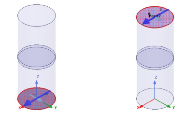
Figure 1: A circular waveguide with a slice of FR4 in the middle. Waveports highlighted on the bottom and top of the cylinder show the coordinate axes (U, V) defined during port setup. Note they are aligned.

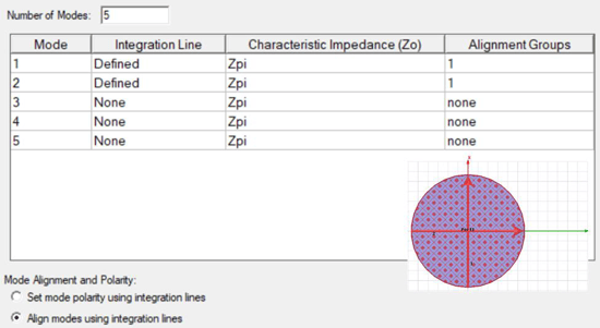
Figure 2: Setting for aligning modes using integration lines. Assign integration lines for first two modes and group them together by assigning ‘alignment group’ 1.

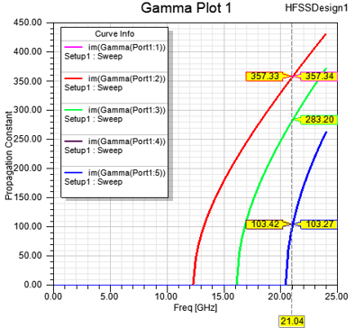
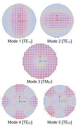
Figure 3: Propagation constants calculated by HFSS for all propagating modes up to 24 GHz for the waveguide in Figure 1. On the right side, note the orientation of modes is dictated by the coordinate axes.

 

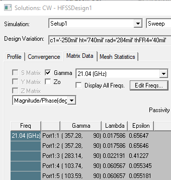
HFSS lists modes in increasing order of gamma. Numerical noise can create ambiguity between degenerate modes. But when we align the modes as explained here, the numerical error doesn’t confuse one mode for the other as shown in the matrix data showing gamma for the first 5 propagating modes. Note the value of gamma for last two modes.